Example – TL for image classification

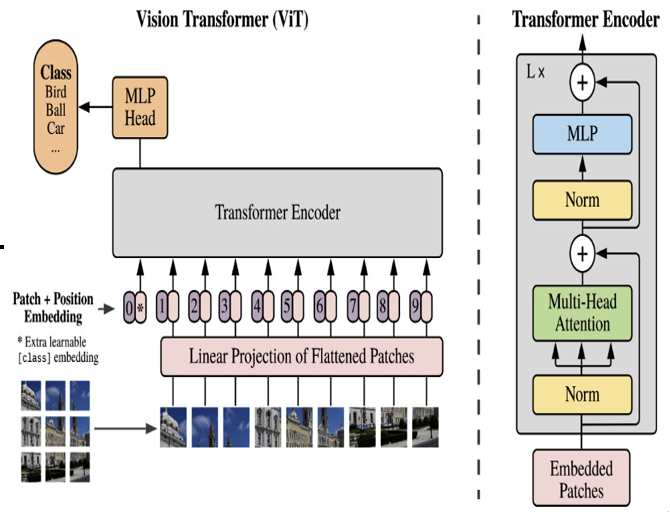
We could take a pre-trained model such as ResNet or the Vision Transformer (shown in Figure 12.10), initially trained on a large-scale image dataset such as ImageNet. This model has already learned to detect various features from images, from simple shapes to complex objects. We can take advantage of this knowledge, fine-tuning the model on a custom image classification task:

Figure 12.10 – The Vision Transformer

The Vision Transformer is like a BERT model for images. It relies on many of the same principles, except instead of text tokens, it uses segments of images as “tokens” instead.

The following code block shows an end-to-end code example of fine-tuning the Vision Transformer on an image classification task. The code should look very similar to the BERT code from the previous section because the aim of the transformers library is to standardize training and usage of modern pre-trained models so that no matter what task you are performing, they can offer a relatively unified training and inference experience.

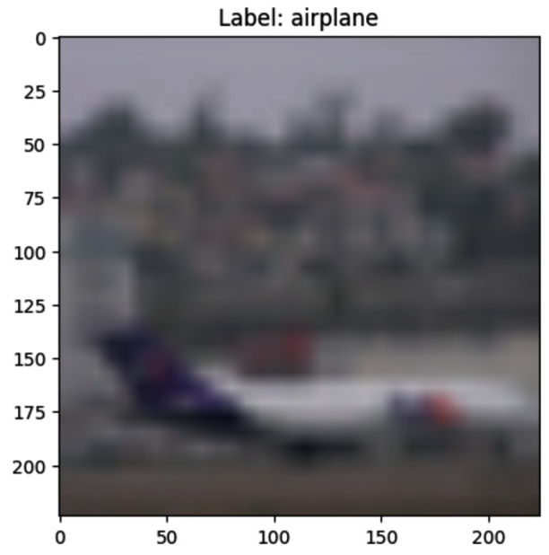
Let’s begin by loading up our data and taking a look at the kinds of images we have (seen in Figure 12.11). Note that we are only going to use 1% of the dataset to show that you really don’t need that much data to get a lot out of pre-trained models!

# Import necessary libraries
from datasets import load_dataset
from transformers import ViTImageProcessor, ViTForImageClassification
from torch.utils.data import DataLoader
import matplotlib.pyplot as plt
import torch
from torchvision.transforms.functional import to_pil_image
# Load the CIFAR10 dataset using Hugging Face datasets
# Load only the first 1% of the train and test sets
train_dataset = load_dataset(“cifar10″, split=”train[:1%]”)
test_dataset = load_dataset(“cifar10″, split=”test[:1%]”)
# Define the feature extractor
feature_extractor = ViTImageProcessor.from_pretrained(‘google/vit-base-patch16-224’)
# Preprocess the data
def transform(examples):
    # print(examples)
    # Convert to list of PIL Images
    examples[‘pixel_values’] = feature_extractor(images=examples[“img”], return_tensors=”pt”)[“pixel_values”]
    return examples
# Apply the transformations
train_dataset = train_dataset.map(
transform, batched=True, batch_size=32
).with_format(‘pt’)
test_dataset = test_dataset.map(
transform, batched=True, batch_size=32
).with_format(‘pt’)

We can similarly use the model using the following code:

Figure 12.11 – A single example from CIFAR10 showing an airplane

Now, we can train our pre-trained Vision Transformer:

# Define the model
model = ViTForImageClassification.from_pretrained(
‘google/vit-base-patch16-224’,
num_labels=10, ignore_mismatched_sizes=True
)
LABELS = [‘airplane’, ‘automobile’, ‘bird’, ‘cat’, ‘deer’, ‘dog’, ‘frog’, ‘horse’, ‘ship’, ‘truck’]
model.config.id2label = LABELS
# Define a function for computing metrics
def compute_metrics(p):
    predictions, labels = p
    preds = np.argmax(predictions, axis=1)
    return {“accuracy”: accuracy_score(labels, preds)}
# Define the training arguments
training_args = TrainingArguments(
    output_dir=’./results’,
    num_train_epochs=5,
    per_device_train_batch_size=4,
    load_best_model_at_end=True,
    # Save and evaluate at the end of each epoch
    evaluation_strategy=’epoch’,
    save_strategy=’epoch’
)
# Define the trainer
trainer = Trainer(
    model=model,
    args=training_args,
    train_dataset=train_dataset,
    eval_dataset=test_dataset
)

Our final model has about 95% accuracy on 1% of the test set. We can now use our new classifier on unseen images, as in this next code block:

from PIL import Image
from transformers import pipeline
# Define an image classification pipeline
classification_pipeline = pipeline(
‘image-classification’,
model=model,
feature_extractor=feature_extractor
)
# Load an image
image = Image.open(‘stock_image_plane.jpg’)
# Use the pipeline to classify the image
result = classification_pipeline(image)

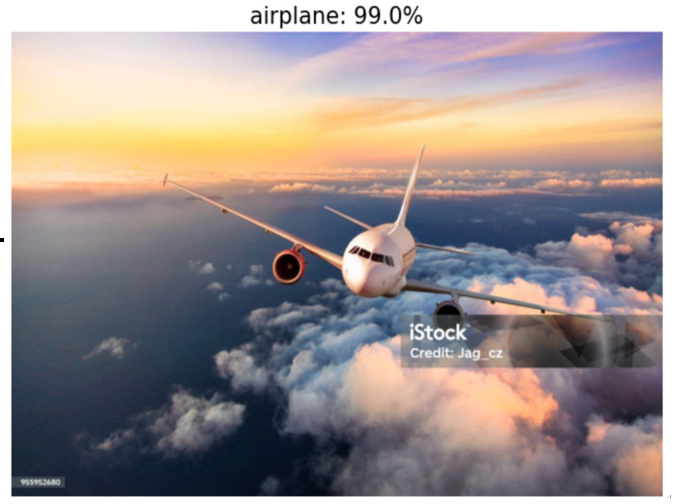
Figure 12.12 shows the result of this single classification, and it looks like it did pretty well:

Figure 12.12 – Our classifier predicting a stock image of a plane correctly

With minimal labeled data, we can leverage TL to turn models off the shelf into powerhouse predictive models.

Summary

Our exploration of pre-trained models gave us insight into how these models, trained on extensive data and time, provide a solid foundation for us to build upon. They help us overcome constraints related to computational resources and data availability. Notably, we familiarized ourselves with image-based models such as VGG16 and ResNet, and text-based models such as BERT and GPT, adding them to our repertoire.

Our voyage continued into the domain of TL, where we learned its fundamentals, recognized its versatile applications, and acknowledged its different forms—inductive, transductive, and unsupervised. Each type, with its unique characteristics, adds a different dimension to our ML toolbox. Through practical examples, we saw these concepts in action, applying a BERT model for text classification and a Vision Transformer for image classification.

But, as we’ve come to appreciate, TL and pre-trained models, while powerful, are not the solution to all data science problems. They shine in the right circumstances, and it’s our role as data scientists to discern when and how to deploy these powerful methods effectively.

As this chapter concludes, the understanding we’ve gleaned of TL and pre-trained models not only equips us to handle real-world ML tasks but also paves the way for tackling more advanced concepts and techniques. By introducing more steps into our ML process (such as pre-training), we are opening ourselves up to more potential errors. Our next chapter will also begin to investigate a hidden side of TL: transferring bias and tackling drift.

Moving forward, consider diving deeper into other pre-trained models, investigating other variants of TL, or even attempting to create your own pre-trained models. Whichever path you opt for, remember—the world of ML is vast and always evolving. Stay curious and keep learning!