Preparing the data for modeling

Having understood the nuances of the bias and fairness definitions, it’s crucial that we give the same attention to our data preparation process. This involves not just the technical transformations but also a thoughtful consideration of the implications of these transformations on fairness.

Feature engineering

We’ve already touched on a few points during EDA, such as combining the three juvenile crime columns. However, before jumping into that, it’s crucial to note that any transformations we apply to our data can introduce or exacerbate biases. Let’s take a detailed look.

Combining juvenile crime data

Combining the juvenile offenses into a single feature is logical for model simplicity. However, this can potentially introduce bias if the three types of juvenile crimes have different recidivism implications based on race. By lumping them together, we could be over-simplifying these implications. Always be wary of such combinations:

# feature construction, add up our three juv columns and remove the original features
compas_df[‘juv_count’] = compas_df[[“juv_fel_count”, “juv_misd_count”, “juv_other_count”]].sum(axis=1)
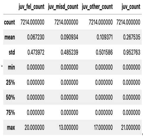
compas_df[[‘juv_fel_count’, ‘juv_misd_count’, ‘juv_other_count’, ‘juv_count’]].describe()

The resulting matrix can be shown in Figure 15.6:

Figure 15.6 – A look at our new columns

One-hot encoding categorical features

We need to convert our categorical variables such as sex, race, and c_charge_degree into a numerical format. Here, using a method such as one-hot encoding can be appropriate. However, it’s essential to remember that introducing too many binary columns can exacerbate issues in fairness if the model gives undue importance to a particular subgroup:
   dummies = pd.get_dummies(compas_df[[‘sex’, ‘race’, ‘c_charge_degree’]], drop_first=True)
   compas_df = pd.concat([compas_df, dummies], a
xis=1)

Standardizing skewed features

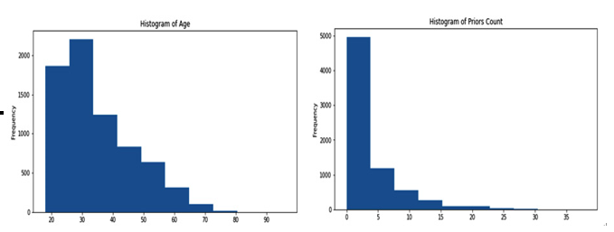
We can easily see that age and priors_count are right-skewed using the following code block and figure. Standardizing these features can help our model train better. Using methods such as log-transform or square root can be useful:

# Right skew on Age
 compas_df[‘age’].plot(
     title=’Histogram of Age’, kind=’hist’, xlabel=’Age’, figsize=(10, 5)
 )
 # Right skew on Priors as well
 compas_df[‘priors_count’].plot(
     title=’Histogram of Priors Count’, kind=’hist’, xlabel=’Priors’, figsize=(10, 5)
 )

Figure 15.7 shows us our two distributions and, more importantly, how much our data is skewed:

Figure 15.7 – Skewed age and priors data can affect our final predictions

If we want to transform our numerical features, we can use a scikit-learn pipeline to run some feature transformations, such as in the following code block:

We can use a scikit-learn pipeline to run a standard scaler like so:
numerical_features = [“age”, “priors_count”]
numerical_transformer = Pipeline(steps=[
    (‘scale’, StandardScal
er())
])

With a transformer in hand, such as the one defined in the preceding code block, we can begin to address skewed data in real time in our ML pipelines.